Get Shift Done: Tips and Tricks
The tabs feature in Google Sheets is a great organizational tool, and it keeps thing neat and tidy. However, sometimes we need a summary spreadsheet, an at-a-glance overview of the data. Or perhaps it’s useful to see a single chart that updates as we add new information. In either case, the quickest solution is to use the =SUMIF function, and it’s easier than it initially appears.
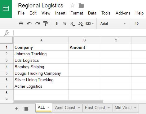
As an example, let’s create a summarized list of the trucking suppliers we pay. First, add a new tab to the Google Sheet that records the column headers that match the information to summarize.
Next, pull in the sum of the total invoiced for the year into the appropriate cell in the “Amount” column. To do so, we use the =“SUMIF” function, which searches for the trucking company name that fits the one in the first row, and then totals the amount owed. The formula looks like this:
=SUMIF(‘West Coast’!A:A,A2,’West Coast’!D:D)
To remember what you are trying to do with the formula, say to yourself: “Sum if West Coast Column A matches Cell A2 then sum the amount in West Coast Column D.”
SUMIF(range, criteria, [sum_range])
Do this for each cell, making sure you match the right tab for each company:
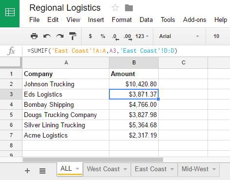
Ta da! Now you have a single sheet, continuously updated, that captures all the detailed tabs below.
Get stories like this one delivered to your in-box weekly: Subscribe to the GSD newsletter.
GSD: Tips and Tricks is brought to you by Xero, the cloud accounting software solution for your small business. With Xero, you can log in anytime, anywhere to get a real-time view of your cash flow and manage your books. Start your free 30-day trial today.